


{This website: Please note: The following article is complete; it has been put into ASCII due to a) space requirement reduction and b) for having thus the possibility to enlarge the fairly small figures. And: special math. symbols are in Unicode. Further: disallow M$-IE 'automatic picture size adaptation'.}
Gabriel Kron's biography here.
Abstract: Equivalent circuits are developed to represent
the Schrödinger amplitude equation for one,
two, and three independent variables in orthogonal curvilinear
coordinate systems. The
networks allow the assumption of any arbitrary potential energy
and may be solved, within any
desired degree of accuracy, either by an a.c. network analyzer, or by
numerical and analytical
circuit methods. It is shown that by varying the impressed frequency
on a network of inductors
and capacitors (or by keeping the frequency constant and varying
the capacitors), it is possible
to find by measurements the eigenvalues, eigenfunctions, and
the statistical mean of various
operators belonging to the system represented. The electrical model may,
of course, be replaced
by an analogous mechanical model containing moving masses and springs.
At first the network
for the one-dimensional wave equation for a single particle in Cartesian
coordinates is developed
in detail, then the general case. A companion paper contains results of a study
made on an a.c.
network analyzer of one-dimensional problems: a potential well, a double barrier,
the harmonic
oscillator, and the rigid rotator. The curves show good agreement,
within the accuracy of the
instruments, with the known eigenvalues, eigenfunctions, and "tunnel" effects.
THE ONE-DIMENSIONAL SCHRÖDINGER
EQUATION
In Cartesian coordinates, the equation is
Three types of equivalent circuits may be
established.
1. The circuit contains positive and negative
resistors and in each state the currents and
voltages are constant in time. The state is
changed by varying the resistances, corresponding
to a change in eigenvalue (energy level).
2. Although negative resistances are available
for use with a network analyzer, in practice it is
more convenient to use a second type of circuit,
in which the positive and negative resistors are
replaced by inductors and capacitors and the d.c.
currents and voltages are replaced by a.c.
currents and voltages of fixed frequency. The use of
the second type of interpretation is equivalent to
multiplying the wave equation by i = √- 1.
In the diagrams to follow, unless otherwise
stated, the inductors (whose reactance at the
fixed frequency is denoted by XL ) may also be
viewed as positive resistances of value XL and the
capacitors (whose reactance is denoted by - XC )
as negative resistances of value - XC.
3. The third type of circuit contains inductors
and capacitors and in each state the currents and
voltages are sinusoidal in time. The state is
changed by varying the frequency of the
impressed voltage.
The basic network concepts will be introduced
in detail in connection with the first type of
circuit (with additional comments on the second
type of interpretation). The third type of model,
although it offers attractive analogies, will be
only cursorily treated.
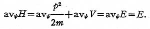
REPRESENTATION OF ENERGY OPERATORS
If the wave equation is multiplied by ∆x and
the operator p = - i ħ∂ /∂x is introduced,
the equation becomes
The three energy operators will be represented
in the following manner:
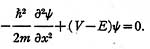
1. The kinetic energy
operator T = p2/ 2m is represented (Fig. 1a) by a
set of equal positive resistors (or inductive coils)
in series extending from -∞ to + ∞. The
impedance of each coil is (2m/ ħ2)∆x.
2. The potential energy operator V is represented (Fig. 1b)
by a set of isolated positive resistors (inductive
coils). The admittance of each coil is V∆x. These
values vary from point to point.
3. The total
energy operator -E is represented (Fig. 1c) by a
set of isolated equal negative resistors (capacitors).
The admittance of each coil is the unknown
quantity E∆x.
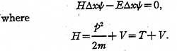
The sum of the two operators T and V forming
the Hamiltonian operator H is represented by the
interconnected network of Fig. 2a. That is, a
summation of energy operators is represented
electrically by an interconnection of the
component networks.
Finally, the sum of the Hamiltonian H and the
total energy -E operators is the resultant
network of Fig. 2b extending from - ∞ to + ∞.
OPERATION ON THE WAVE FUNCTION ψ
The wave function ψ will be assumed to be
represented (Fig. 3) by the differences of
potential (1) appearing between the junctions of the
three types of coils and the ground connection
(impedanceless wire). The function ψ varies
along ψ' but is constant in time. An
eigenfunction ψ' of H depends on the time as follows:
ψ' = ψ exp [-i(E/ ħ)t].
The differences of potentials appearing
between two junctions are
∆ψ = (∂ψ/ ∂x )∆x + ...
where higher order terms in the Taylor series
development are neglected.
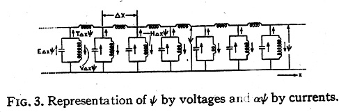
The result of the operation αψ or βψ (where α
and α are operators) is represented by currents
flowing in the respective component networks, as
shown in Fig. 3. In particular:
1. The currents
flowing in the capacitors are E∆xψ.
2. The currents flowing in the vertical inductors
are V∆xψ.
3. The currents flowing in the horizontal
inductors are
β∆ψ = (ħ2/ 2m)(∂ψ/∂x).
4. The currents flowing out of the horizontal inductors at
their junctions are
∆(β∆ψ) = (ħ2/2m)(∂2ψ/∂x2)
representing (-T∆xψ).
Since E∆xψ represents the currents flowing in
the capacitors and H∆xψ = (T+ V)∆xψ those in
the inductors, the equation H∆xψ = E∆xψ simply
states Kirchhoffs second law, that at each of the
junctions of four coils the currents flowing into
the positive resistors (inductors) are equal to
the currents coming from the negative resistors
(capacitors).
Both the voltages and currents appear as
standing waves. When the space distribution of
ψ is such that it attenuates, the network may be
terminated at any point by an equivalent
impedance. When ψ does not attenuate the circuit
may be terminated by a short circuit at any point
of zero voltage, or by an open circuit at any point
of zero current. These points are easily determined
on the a.c. network analyzer by trial.
It should be noted that the equivalent circuit
introduces an indeterminacy between quantities
measured in the vertical coils and those in the
horizontal coils. If, for instance, the vertical
voltage ψ is known at a certain value of x, say x0,
then the horizontal current
(ħ2/2m)(∂ψ/∂x)
is not known at that particular x0, only at some indeterminate
value between x0 and x0+∆x/2 or
x0-∆x/2.
EIGENVALUES AND EIGENFUNCTIONS
Let it be assumed as an example that the V
function is a potential well (Fig. 4a). Then in the
network the corresponding positive resistances
assume either a constant or a zero value as shown
in Fig. 4b. In practice it is sufficient to extend the
network to, say, twice the width of the potential
well on either side.
Let now a d.c. (or a.c.) generator be inserted
anywhere in the network parallel with one of the
negative resistances (inductors), as shown. If the
values of all the negative resistances -E∆x
(capacitors) are simultaneously varied by the
same amount, it will be found that the current
(reactive current) in the generator varies and at
some value of E∆x becomes zero.
It should be noted that while a current (reactive
current) flows in the generator the circuit does
not satisfy the differential equation, since at one
point in the network (where the generator is
connected) the currents do not add up to zero (as
required by the equation) but to the generator
current. That is, while a current flows in the
generator, the voltages ψ do not represent
solutions of the differential equation. Hence, only
those network conditions are of interest in which
the generator current is zero.
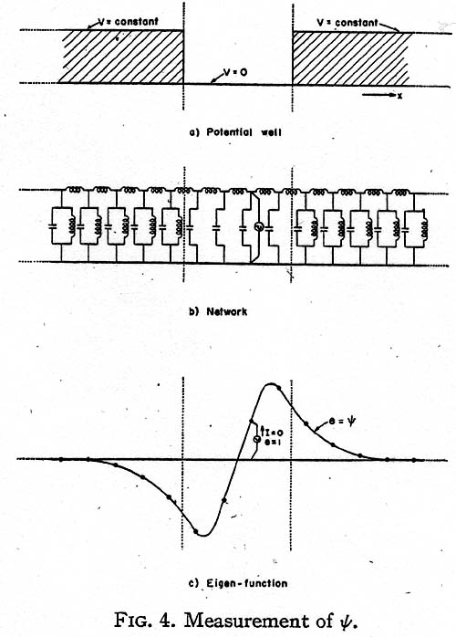
Now a value E of the negative resistances, at
which the generator current becomes zero, represents
a state at which the circuit is self-supporting
and has a continuous existence of its own without
the presence of the generator, as the negative
resistances just supply the energy consumed by
the positive resistances. (If the circuit contains
inductors and capacitors, the circuit is a resonant
circuit and it oscillates at its basic frequency.)
E is then an eigenvalue En, while the voltage
distribution across the capacitors (Fig. 4c) gives
the corresponding eigenfunction ψn.
When the generator current is positive the
circuit draws energy from the source, and when
the current is negative the circuit pumps back
energy into the source. At zero generator current
the circuit neither gives nor takes energy, and
theoretically the generator may be removed. All
values of E at which the current crosses the axes
and becomes zero are eigenvalues of the equation
and the corresponding voltage distribution curves
are eigenfunctions. When the energy level E
overflows the well, the discrete spectrum of
eigenvalues changes into a continuous spectrum
and the generator current is zero at all greater
values of E.
When the energy E changes sign, the negative
resistances become positive resistances and at no
value of -E may the circuit be self-supporting
(as it contains only positive resistances). That is,
the equation has no negative eigenvalues.
THE STATISTICAL MEAN OF OPERATORS
To bring the measurements at the different
energy levels to the same base, it is necessary to
normalize the measured ψ values so that the new
values of ψ satisfy the equation
The measured ψ functions are normalized by
plotting the square of ψ. If the area under the
curve is 1/N2, all values of ψ are multiplied by N.
Then Nψ is the normalized ψ. (Actually N may
contain an arbitrary phase eiγ .)
The statistical mean of an operator α for a
state ψ is defined as
Since (a∆x)ψ is a current (reactive current)
flowing through an admittance, ψ*(a∆x)ψ is the
power (reactive power) in a single admittance.
Hence the total power in a complete set of
similar admittances, namely,
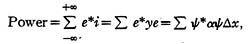
represents the statistical mean of the
corresponding energy operator. That is:
1. The total
power in all the vertical negative resistors is the
average value of E. (That is, E itself, since ψ is an
eigenfunction of H).
2. The total power in all the
vertical resistors is the average value of the
potential energy V.
3. The total power in all the
horizontal resistors is the same as the total power
in the vertical units, representing the average of
the kinetic energy T = p2/ 2m.
That is, the total power in all positive resistors
is the same as the total power in all the negative
resistors, or
THE THIRD MODEL
Let the wave equation be divided by iωc, where
ωc = √ω = (E/ ħ)½,
and multiplied by ∆x:
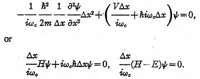
In the present case:
1. The kinetic energy operator T is represented
(Fig. 5) by a set of equal inductors in series,
whose inductance L1 is (2m/ ħ2)∆x.
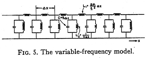
2. The potential energy operator V is represented by a set
of unequal coils in parallel, whose inductance L2
is 1/ V∆x.
3. The total energy operator - E is
represented by a set of equal capacitors in
parallel whose capacitance is now ħ∆x. (In
the second model the capacitance was the
unknown E∆x.)
The operand ψ is again represented by voltages
and the result of the operation αψ by the same
currents as in the first model. Their variation in
time now is sinusoidal,
with 2 π fc = ωc.
Instead of varying the magnitude of the
capacitors, now the frequency of the generator is
varied, thereby varying the admittance of the
capacitors, ħωc = E (and those of the inductors).
Again when the generator current becomes zero
the circuit is oscillatory and self-supporting and
the network represents a stationary solution of
the equation. The corresponding eigenvalue is
E = ħω = ħ(ωc )2,
rather than ħωc, because of the
simultaneous variation of the reactance of the
inductive coils. The eigenfunctions ψ of the model
and of the equation are, however, identical.
As the currents in the horizontal inductors are
(ħ2/2miωc )∂ψ/ ∂x,
the results of an operation on ψ
by the momentum operator p = (ħ / i)∂/ ∂x are
these currents divided by ħ2/ 2mωc.
Hence, in the
third model the momentum operator p may be
represented by a set of equal horizontal coils with
inductance L = ∆x/ħωc.
One slight disadvantage of this third model is
that as the energy E changes sign, the reactance
of the capacitor jωcħ cannot change signs. Since in
most cases no eigenvalues exist in the negative
energy range, this disadvantage is of little
consequence. Of course, the second model with fixed
frequency and variable capacitors works in all
cases, since the capacitors simply become
inductors when E changes sign.
THE FREE PARTICLE IN ONE DIMENSION
An interesting special case occurs when the
potential V is zero everywhere. The one-dimensional
equivalent circuit of such a free
particle is a conventional transmission line
extending to infinity in both directions (Fig. 6) in
which the series inductance is 2m ∆x/ ħ2 and the
shunt capacitor is ħ∆x.
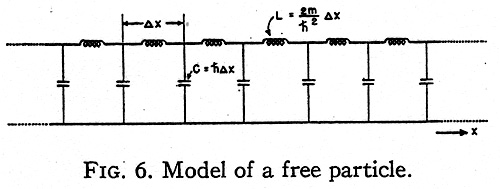
It is well known that such a transmission line
may maintain a standing wave at any frequency
ψ=ωc between zero and infinity drawing no current
from the generator. That is, the positive energy
values form a continuous spectrum. If the
transmission line is considered as the second type of
model with variable capacitors, then at negative
energy values E the capacitors also become
inductors and the line cannot maintain a standing
wave. The corresponding free particle also has no
eigenvalue at the negative energy levels.
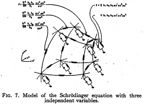
MODELS ALONG CURVILINEAR AXES
The three-dimensional Schrödinger equation
for a single particle is
where ∇2
is the Laplacian operator in curvilinear coordinates.
In order to establish a physical model for it,
it is necessary to change it to a tensor density
equation. (2)
The above equation in orthogonal
curvilinear coordinates may be changed to a
tensor density form by multiplying it by
h1h2h3 = √g giving
If the equation is multiplied through by
∆u1∆u2∆u3,
it represents the surface integral of
grad ψ around the six faces of a cube of space with
volume
h1h2h3∆u1∆u2∆u3.
The width ∆uα may be
arbitrary and different in the three directions.
The corresponding equivalent circuit is shown
in Fig. 7. For a free particle (V=0) it represents
a generalization of the conventional one-dimen-
sional transmission line to three dimensions.
NOTES AND REFERENCES
(1) It is possible to establish in one dimension a dual
network in which ψ is represented by a current instead of
a voltage. However, in two and three dimensions the dual
networks require ideal transformers.
(2) G. Kron, Proc. I. R. E, 32, 289-299 (May, 1944).
Last updated : Sept. 5, 2003 - 22:44 CET